
Overview
This lesson utilizes a video snippet capturing 8 months of underwater footage from the Southern Hydrate Ridge, obtained by the Ocean Observatories Initiative (OOI)RCA’s digital still camera. Hydrate Ridge is populated by large communities of giant sulfide-oxidizing bacteria (Beggiatoa) and of the symbiotic vesicomyid clam Calyptogena pacifica and Calyptogena kilmeri, which are associated with surficial hydrate deposits and high fluid flow. The presence of the RCA digital still camera allows us to study the variations of the coverage of this biogenic sediment at a very fine scale. For those interested in learning more, please refer to Antje Boetius and Erwin Suess, “Hydrate Ridge: a natural laboratory for the study of microbial life fueled by methane from near-surface gas hydrates,”. The primary objective is to analyze the changes in biogenic (living organisms) to inert (non-living) sediment ratios over time, offering insights into the seafloor ecosystem dynamics. The workflow involves downloading a video and extracting frames. Image processing techniques, such as CLAHE and HSV conversion, are used to preprocess frames, and KMeans clustering is applied for segmentation, identifying clusters representing different sediment types (biogenic and inert). The notebook quantifies the percentage cover of each cluster over time, producing data that is visualized using stacked bar charts. These charts illustrate the temporal changes in sediment ratios, and linear regression is applied to further quantify these trends. The output includes segmented images, cluster information (colors and percentage cover), stacked bar charts, and linear regression results, providing a comprehensive view of sediment dynamics in the study area.
Learning Objectives:
By the end of this section, you will:
Download and process video data within a Google Colab environment.
Apply image processing techniques, including CLAHE and HSV conversion for preprocessing the frames.
Apply image processing techniques, including CLAHE and HSV conversion for preprocessing the frames.
Segment images using KMeans clustering, identifying regions with distinct visual properties.
Make decisions about the meaning and science context behind clusters.
Quantify the percentage coverage of different sediment types over time.
Interpret the patterns identified in the data and draw conclusions about sediment dynamics in the study area.
Libraries Overview
Here’s a quick overview of the most important new imports used in the KMeans segmentation lesson:
sklearn.cluster (KMeans): A machine learning tool for clustering data, useful in tasks like color quantization or image segmentation.
skimage.segmentation (slic): A function for segmenting images using a superpixel approach, useful for simplifying image data for analysis.
skimage.util (img_as_float): Converts image data to floating-point representation, often needed for processing images in scientific computations.
Key Concepts
Superpixels
Superpixels are groups of pixels with similar characteristics that are treated as a single entity. In image segmentation, superpixels help simplify an image by reducing the number of pixels that need to be analyzed, making algorithms more efficient. The slic function from the skimage library is used to generate superpixels. This helps in dividing the image into meaningful regions, which makes subsequent analysis, like clustering, more effective.
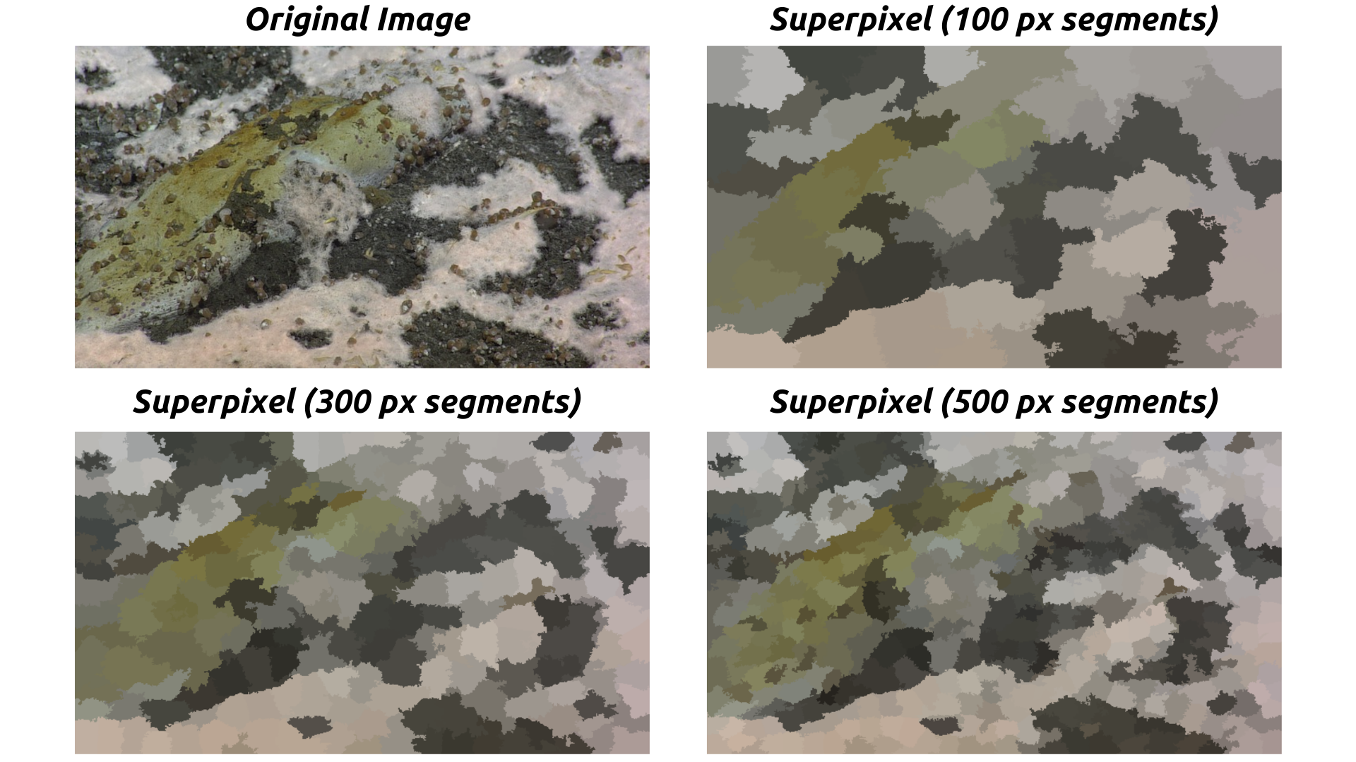
Figure 1:Example of Superpixel Segmentation. Credit: NSF/UW/CSSF
KMeans Clustering
KMeans is a clustering algorithm used to partition data into distinct groups based on similarity. In the context of image segmentation, KMeans helps in grouping pixels into clusters based on their color and intensity values. This allows us to differentiate between areas of biogenic and inert sediments by assigning them into separate clusters, which can then be quantified for analysis.
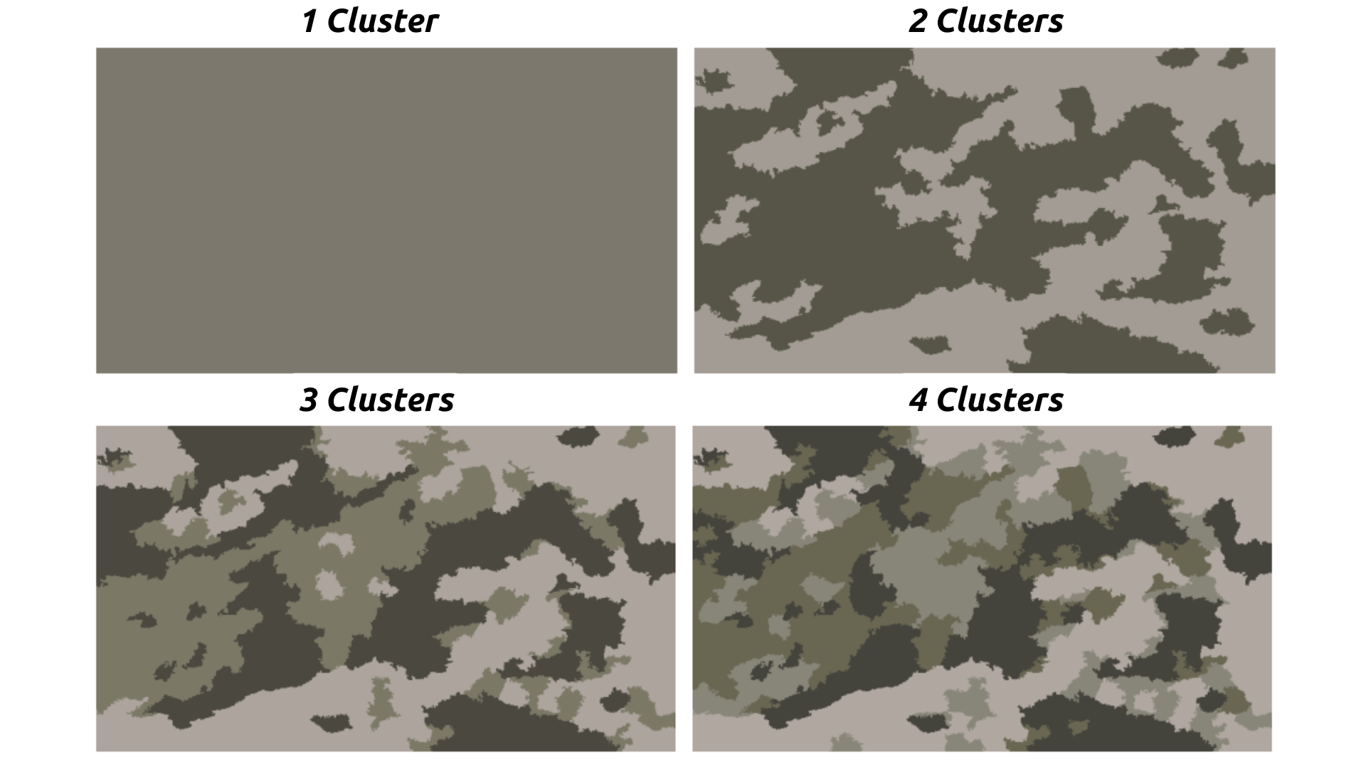
KMeans Clustering applied to an Underwater Image. Credit: NSF/UW/CSSF
CLAHE (Contrast Limited Adaptive Histogram Equalization)
CLAHE is an image enhancement technique that improves the contrast of images, especially in areas with poor lighting. It is particularly useful for underwater footage, where visibility can be challenging due to the presence of particulate matter and variations in light. CLAHE is uniquely suited to biogenic sediment analysis for camera systems set at an oblique or in heavily shadowed environments. This is because often times color and value are the most important distinctions between sediment types, and applying image-wide brightness adjustments will not preserve the difference in color and will miss a lot. By enhancing the contrast, CLAHE makes it easier for segmentation algorithms, like KMeans, to identify different features in the image more effectively.
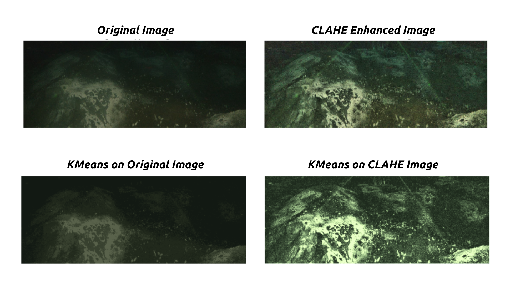
Figure 3:Effect of CLAHE on Underwater Image. Credit: NSF/UW/CSSF
!pip install moviepy scikit-image scikit-learn
Requirement already satisfied: moviepy in /usr/local/lib/python3.11/dist-packages (1.0.3)
Requirement already satisfied: scikit-image in /usr/local/lib/python3.11/dist-packages (0.25.1)
Requirement already satisfied: scikit-learn in /usr/local/lib/python3.11/dist-packages (1.6.1)
Requirement already satisfied: decorator<5.0,>=4.0.2 in /usr/local/lib/python3.11/dist-packages (from moviepy) (4.4.2)
Requirement already satisfied: imageio<3.0,>=2.5 in /usr/local/lib/python3.11/dist-packages (from moviepy) (2.37.0)
Requirement already satisfied: imageio_ffmpeg>=0.2.0 in /usr/local/lib/python3.11/dist-packages (from moviepy) (0.6.0)
Requirement already satisfied: tqdm<5.0,>=4.11.2 in /usr/local/lib/python3.11/dist-packages (from moviepy) (4.67.1)
Requirement already satisfied: numpy>=1.17.3 in /usr/local/lib/python3.11/dist-packages (from moviepy) (1.26.4)
Requirement already satisfied: requests<3.0,>=2.8.1 in /usr/local/lib/python3.11/dist-packages (from moviepy) (2.32.3)
Requirement already satisfied: proglog<=1.0.0 in /usr/local/lib/python3.11/dist-packages (from moviepy) (0.1.10)
Requirement already satisfied: scipy>=1.11.2 in /usr/local/lib/python3.11/dist-packages (from scikit-image) (1.13.1)
Requirement already satisfied: networkx>=3.0 in /usr/local/lib/python3.11/dist-packages (from scikit-image) (3.4.2)
Requirement already satisfied: pillow>=10.1 in /usr/local/lib/python3.11/dist-packages (from scikit-image) (11.1.0)
Requirement already satisfied: tifffile>=2022.8.12 in /usr/local/lib/python3.11/dist-packages (from scikit-image) (2025.1.10)
Requirement already satisfied: packaging>=21 in /usr/local/lib/python3.11/dist-packages (from scikit-image) (24.2)
Requirement already satisfied: lazy-loader>=0.4 in /usr/local/lib/python3.11/dist-packages (from scikit-image) (0.4)
Requirement already satisfied: joblib>=1.2.0 in /usr/local/lib/python3.11/dist-packages (from scikit-learn) (1.4.2)
Requirement already satisfied: threadpoolctl>=3.1.0 in /usr/local/lib/python3.11/dist-packages (from scikit-learn) (3.5.0)
Requirement already satisfied: charset-normalizer<4,>=2 in /usr/local/lib/python3.11/dist-packages (from requests<3.0,>=2.8.1->moviepy) (3.4.1)
Requirement already satisfied: idna<4,>=2.5 in /usr/local/lib/python3.11/dist-packages (from requests<3.0,>=2.8.1->moviepy) (3.10)
Requirement already satisfied: urllib3<3,>=1.21.1 in /usr/local/lib/python3.11/dist-packages (from requests<3.0,>=2.8.1->moviepy) (2.3.0)
Requirement already satisfied: certifi>=2017.4.17 in /usr/local/lib/python3.11/dist-packages (from requests<3.0,>=2.8.1->moviepy) (2025.1.31)
Source
import os
import cv2
import numpy as np
import requests
import matplotlib.pyplot as plt
import matplotlib.patches as patches
import plotly.express as px
from moviepy.editor import VideoFileClip, ImageSequenceClip
from sklearn.cluster import KMeans
from collections import Counter
from skimage.segmentation import slic
from skimage.util import img_as_float
from IPython.display import HTML, display
from base64 import b64encode
import ipywidgets as widgets
import pandas as pd
WARNING:py.warnings:/usr/local/lib/python3.11/dist-packages/moviepy/video/io/sliders.py:61: SyntaxWarning: "is" with a literal. Did you mean "=="?
  if event.key is 'enter':
Set and Define Functions
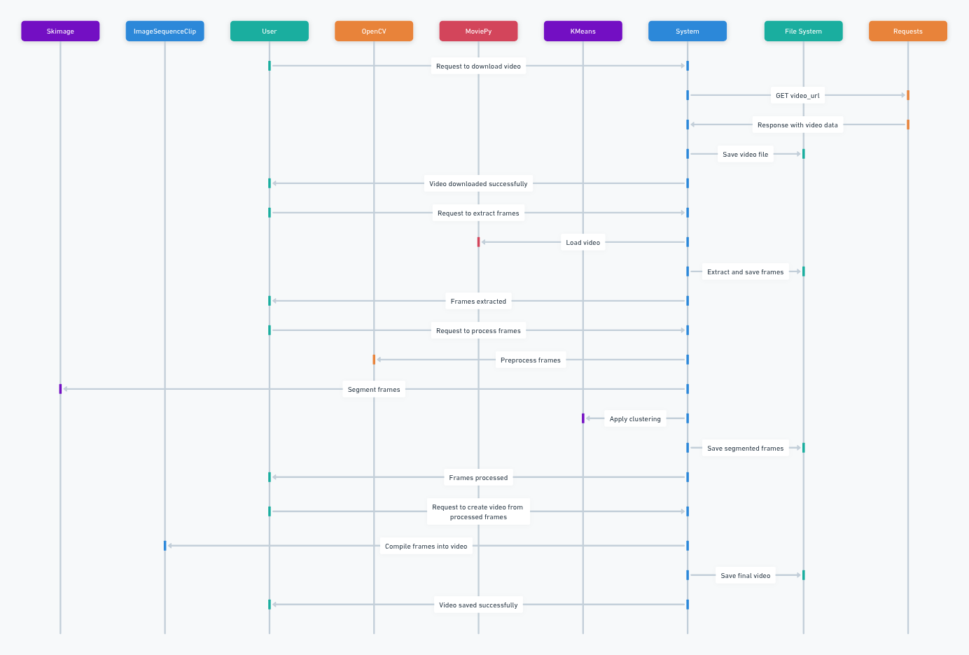
Figure 4:A diagram showing the I/O of the following functions Credit: Carter
Run the following cell to set up your notebook for the clustering workflow. See the figure above to understand the flow of the following functions.
def download_video(video_url, save_path):
    response = requests.get(video_url, stream=True)
    if response.status_code == 200:
        with open(save_path, 'wb') as f:
            for chunk in response.iter_content(chunk_size=1024):
                f.write(chunk)
        print(f"Video downloaded successfully and saved to: {save_path}")
    else:
        print(f"Failed to download video. Status code: {response.status_code}")

# Function to extract frames from a local video file
def extract_frames_from_video(video_path, output_dir, frame_rate=10, width=1024, height=1024):
    # Create the output directory if it doesn't exist
    os.makedirs(output_dir, exist_ok=True)

    # Load the video using moviepy
    clip = VideoFileClip(video_path)

    # Extract frames at the specified rate and resolution
    for i, frame in enumerate(clip.iter_frames(fps=frame_rate)):
        # Resize the frame
        resized_frame = cv2.resize(frame, (width, height))

        # Save the frame
        frame_path = os.path.join(output_dir, f'frame_{i:04d}.png')
        cv2.imwrite(frame_path, resized_frame)

    print(f"Frames extracted and saved to: {output_dir}")

# Function to apply KMeans clustering to an image
def apply_kmeans(image, n_clusters, kmeans_model=None):
    pixel_values = image.reshape((-1, 3))
    pixel_values = np.float32(pixel_values)

    if kmeans_model is None:
        kmeans = KMeans(n_clusters=n_clusters, random_state=42)
        kmeans.fit(pixel_values)
    else:
        kmeans = kmeans_model

    labels = kmeans.predict(pixel_values)
    segmented_image = kmeans.cluster_centers_[labels]
    segmented_image = segmented_image.reshape(image.shape)
    segmented_image = np.uint8(segmented_image)

    return segmented_image, labels, kmeans

# Function to preprocess an image using CLAHE and HSV conversion
def preprocess_image(image):
    image_cropped = image[-400:, :, :]
    hsv_image = cv2.cvtColor(image_cropped, cv2.COLOR_BGR2HSV)
    clahe = cv2.createCLAHE(clipLimit=2.0, tileGridSize=(8, 8))
    hsv_image[:, :, 2] = clahe.apply(hsv_image[:, :, 2])
    preprocessed_image = cv2.cvtColor(hsv_image, cv2.COLOR_HSV2BGR)
    return preprocessed_image

# Function to segment an image using SLIC algorithm
def segment_image(image, n_segments):
    image_float = img_as_float(image)
    segments = slic(image_float, n_segments=n_segments, compactness=10, start_label=0)
    return segments

# Function to process an image, apply KMeans, save output, and add cluster information
def process_and_save_image(image, kmeans_model, filename, output_dir):
    image_cropped = preprocess_image(image)
    segments = segment_image(image_cropped, n_segments=500)
    segmented_image, labels, _ = apply_kmeans(image_cropped, n_clusters=4, kmeans_model=kmeans_model)
    label_counts = Counter(labels)
    cluster_info = []
    total_pixels = image_cropped.shape[0] * image_cropped.shape[1]
    cluster_hsv_values = kmeans_model.cluster_centers_
    for i in range(4):
        cluster_percentage = (label_counts[i] / total_pixels) * 100
        cluster_hsv = cluster_hsv_values[i]
        cluster_info.append(f"Cluster {i}: {label_counts[i]} pixels ({cluster_percentage:.2f}%) - HSV: ({cluster_hsv[0]:.2f}, {cluster_hsv[1]:.2f}, {cluster_hsv[2]:.2f})")

    segmented_image_bgr = cv2.cvtColor(segmented_image, cv2.COLOR_HSV2BGR)
    output_image_path = os.path.join(output_dir, filename)
    cv2.imwrite(output_image_path, segmented_image_bgr)

    output_txt_path = os.path.join(output_dir, filename.rsplit('.', 1)[0] + '_clusters.txt')
    with open(output_txt_path, 'w') as f:
        f.write("\n".join(cluster_info))

    for i, info in enumerate(cluster_info):
        text_position = (10, 30 + i * 20)
        cv2.putText(segmented_image_bgr, info, text_position, cv2.FONT_HERSHEY_SIMPLEX, 0.6, (255, 255, 255), 2)

    return segmented_image_bgr

# Function to process all frames and segment them
def process_frames(output_dir):
    frames = os.listdir(output_dir)
    if not frames:
        print("No frames available for processing.")
        return

    # Process the first image to initialize KMeans model
    first_image_path = os.path.join(output_dir, frames[0])
    first_image = cv2.imread(first_image_path)
    first_image_cropped = preprocess_image(first_image)
    segmented_image, labels, kmeans_model = apply_kmeans(first_image_cropped, n_clusters=4)

    # Process all frames and store processed frames in a list
    processed_frames_list = []  # Create a list to store processed frames
    for filename in frames:
        if filename.endswith(('.png', '.jpg', '.jpeg')):
            image_path = os.path.join(output_dir, filename)
            image = cv2.imread(image_path)
            processed_frame = process_and_save_image(image, kmeans_model, filename, output_dir)
            processed_frames_list.append(processed_frame)  # Append processed frame to the list

    print("Segmentation completed, results saved.")
    return processed_frames_list  # Return the list of processed frames

# Function to create a video from processed frames
def create_video_from_frames(frames, output_video_path, fps=10):
    clip = ImageSequenceClip([cv2.cvtColor(frame, cv2.COLOR_BGR2RGB) for frame in frames], fps=fps)
    clip.write_videofile(output_video_path, codec='libx264')
    print(f"Video saved to: {output_video_path}")
video_url = "https://github.com/atticus-carter/cv/raw/refs/heads/main/videos/output_video_8.avi"
video_path = "/content/2022SHRSubset.avi"
frames_output_dir = "/content/frames"  # Change to your desired output directory
segmented_video_output_path = "/content/segmented_videos/segmented_video.mp4"

os.makedirs(os.path.dirname(segmented_video_output_path), exist_ok=True)
os.makedirs(frames_output_dir, exist_ok=True)
os.makedirs("/content/segmented_videos", exist_ok=True)

# Download the video
download_video(video_url, video_path)

# Extract frames from local video
extract_frames_from_video(video_path, frames_output_dir)

# Process frames for segmentation
processed_frames = process_frames(frames_output_dir)

# Create video from processed frames
create_video_from_frames(processed_frames, segmented_video_output_path)
Video downloaded successfully and saved to: /content/2022SHRSubset.avi
Frames extracted and saved to: /content/frames
Segmentation completed, results saved.
Moviepy - Building video /content/segmented_videos/segmented_video.mp4.
Moviepy - Writing video /content/segmented_videos/segmented_video.mp4
Moviepy - Done !
Moviepy - video ready /content/segmented_videos/segmented_video.mp4
Video saved to: /content/segmented_videos/segmented_video.mp4
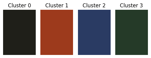
Displaying Cluster Colors with Original Image and Video Frame
This section defines a function to display the cluster colors, original image, and a video frame clip. It reads cluster information from a text file, extracts HSV color values, loads the corresponding image, and creates color swatches using Matplotlib to visualize the clusters. It then displays the swatches along with the original and clustered images using Plotly for interactive viewing.
Source
def display_cluster_colors_with_image(cluster_file_path, image_path, video_path):
    """Displays the colors of the clusters visually from a cluster text file,
    along with the original image and an original video frame clip using Plotly's imshow."""

    # Extract and display the first frame from the video
    clip = VideoFileClip(video_path)
    first_frame = clip.get_frame(0)  # Get the first frame

    # Cut it down to the bottom 400 pixels
    first_frame_cropped = first_frame[-400:, :, :]

    # Save the cropped image
    os.makedirs("/content", exist_ok=True)
    cv2.imwrite("/content/cropped_image.png", first_frame_cropped)

    # Convert BGR to RGB for display with plotly
    image_rgb = cv2.cvtColor(first_frame_cropped, cv2.COLOR_BGR2RGB)

    # Display the original image clip using Plotly
    fig_original = px.imshow(image_rgb)
    fig_original.update_layout(title="Original Image Clip")
    fig_original.show()

    cluster_file = os.path.join(cluster_file_path, "frame_0000_clusters.txt")
    with open(cluster_file, 'r') as f:
        lines = f.readlines()

    hsv_colors = []
    for line in lines:
        if 'HSV' in line:
            hsv_str = line.split('HSV: ')[1].strip('()\n').split(',')
            hsv_colors.append([float(x.strip()) for x in hsv_str])

    # Load the image
    image_file = os.path.join(image_path, "frame_0000.png")
    image2 = cv2.imread(image_file)
    image_rgb_clust = cv2.cvtColor(image2, cv2.COLOR_BGR2RGB)  # Convert to RGB

    # Create color swatches using matplotlib
    fig, ax = plt.subplots(1, len(hsv_colors), figsize=(5, 2))

    for i, hsv_color in enumerate(hsv_colors):
        bgr_color = cv2.cvtColor(np.uint8([[hsv_color]]), cv2.COLOR_HSV2BGR)[0][0]
        rgb_color = bgr_color[::-1]

        rect = patches.Rectangle((0, 0), 1, 1, facecolor=tuple(rgb_color / 255.0))
        ax[i].add_patch(rect)
        ax[i].axis('off')
        ax[i].set_title(f'Cluster {i}')

    plt.tight_layout()

    # Display the clustered image using Plotly's imshow
    fig_image = px.imshow(image_rgb_clust)
    fig_image.update_layout(title="Clustered Image")

    # Show both plots (color swatches and image)
    fig_image.show()
    plt.show()


cluster_file_path = frames_output_dir
image_path = frames_output_dir
video_path = video_path
frames_output_dir = frames_output_dir
segmented_video_output_path = segmented_video_output_path
display_cluster_colors_with_image(cluster_file_path, image_path, video_path)
Displaying the Segmented Video
This section defines a function to display the segmented video within the notebook. It reads the video file, encodes it in base64 format, and then generates an HTML video tag to embed the video for playback.
def show_video(video_path, width=600):
  mp4 = open(video_path,'rb').read()
  data_url = "data:video/mp4;base64," + b64encode(mp4).decode()
  return HTML("""
  <video width="{0}" controls>
        <source src="{1}" type="video/mp4">
  </video>
  """.format(width, data_url))

show_video(segmented_video_output_path)Generating and Displaying Stacked Bar Chart of Cluster Coverage Over Time
This section focuses on quantifying the cluster coverage over time and visualizing it. It extracts cluster percentage data from the text files generated during segmentation, creates a Pandas DataFrame to store the data, and then uses Plotly to generate a stacked bar chart showing the percentage cover of each cluster across the video frames.
Source
import plotly.graph_objs as go
import pandas as pd
import os  # Make sure os module is imported

# Gather cluster data from text files
frame_numbers = []
cluster_percent_cover = {
    'Cluster 0': [],
    'Cluster 1': [],
    'Cluster 2': [],
    'Cluster 3': []
}

# Get a list of all image files in the frames directory
frames_dir = frames_output_dir
image_files = [f for f in os.listdir(frames_dir) if f.endswith(('.png', '.jpg', '.jpeg'))]  # Get all image files

# Parse cluster data from corresponding text files
for i in range(len(image_files)):  # Iterate over all image files
    frame_number = int(image_files[i].split('_')[1].split('.')[0])  # Extract frame number from filename
    txt_file_path = os.path.join(frames_dir, f"frame_{str(frame_number).zfill(4)}_clusters.txt")
    if not os.path.exists(txt_file_path):
        print(f"Warning: could not find {txt_file_path}")
        continue

    with open(txt_file_path, 'r') as file:
        data = file.readlines()
        # Extract cluster percentages (assuming 4 clusters)
        try:
            cluster_percent_cover['Cluster 0'].append(float(data[0].split('(')[1].split('%')[0].strip()))
            cluster_percent_cover['Cluster 1'].append(float(data[1].split('(')[1].split('%')[0].strip()))
            cluster_percent_cover['Cluster 2'].append(float(data[2].split('(')[1].split('%')[0].strip()))
            cluster_percent_cover['Cluster 3'].append(float(data[3].split('(')[1].split('%')[0].strip()))
        except IndexError:
            print(f"Warning: insufficient data in {txt_file_path}")
            continue

    frame_numbers.append(frame_number)

# Create a DataFrame for easier plotting
df = pd.DataFrame(cluster_percent_cover, index=frame_numbers)
df.index.name = 'Frame Number'

# Plotting the stacked bar chart using Plotly
fig = go.Figure()
fig.add_trace(go.Bar(
    x=df.index,
    y=df['Cluster 0'],
    name='Cluster 0'
))
fig.add_trace(go.Bar(
    x=df.index,
    y=df['Cluster 1'],
    name='Cluster 1'
))
fig.add_trace(go.Bar(
    x=df.index,
    y=df['Cluster 2'],
    name='Cluster 2'
))
fig.add_trace(go.Bar(
    x=df.index,
    y=df['Cluster 3'],
    name='Cluster 3'
))

fig.update_layout(
    barmode='stack',
    title='Percent Cover of Each Cluster Over Time',
    xaxis_title='Frame Number',
    yaxis_title='Percent Cover',
    template='plotly_white',
    hovermode='x unified',
    legend_title='Clusters'
)

fig.show()
Interactive Cluster Renaming and Merging
This section enables interactive renaming of clusters and merging of data based on the new names. It uses ipywidgets to create text boxes for users to input new names for each cluster. When a button is clicked, it merges the cluster data in the DataFrame based on the assigned new names, effectively combining clusters represented by the same name into a single category. It saves the result in the mergeddf dataframe.
Source
# Create text boxes for renaming clusters
rename_widgets = [
    widgets.Text(value=f'Cluster {i}', description=f'Cluster {i}:') for i in range(4)
]

# Display widgets for renaming
print("Enter new names for the clusters:")
for w in rename_widgets:
    display(w)

# Button to confirm changes
button = widgets.Button(description="Apply Changes")
output = widgets.Output()

def on_button_click(b):
    with output:
        output.clear_output()  # Clear previous output
        # Get new cluster names
        new_names = [w.value for w in rename_widgets]

        # Merge clusters if they have the same name
        unique_names = list(set(new_names))
        merged_clusters = {name: [] for name in unique_names}

        # Plotting the updated clusters
        frames_dir = frames_output_dir # Path to the directory containing the frames
        if not os.path.exists(frames_dir):
            print(f"Error: Frames directory {frames_dir} does not exist.")
            return

        image_files = [f for f in os.listdir(frames_dir) if f.endswith(('.png', '.jpg', '.jpeg'))]  # Get all image files

        frame_numbers = []

        # Parse cluster data from corresponding text files
        for i in range(len(image_files)):  # Iterate over all image files
            frame_number = int(image_files[i].split('_')[1].split('.')[0])  # Extract frame number from filename
            txt_file_path = os.path.join(frames_dir, f"frame_{str(frame_number).zfill(4)}_clusters.txt")
            if not os.path.exists(txt_file_path):
                continue

            with open(txt_file_path, 'r') as file:
                data = file.readlines()
                # Extract cluster percentages (assuming 4 clusters)
                try:
                    cluster_data = [float(data[j].split('(')[1].split('%')[0].strip()) for j in range(4)]
                except IndexError:
                    continue

                # Merge clusters based on new names
                for j, name in enumerate(new_names):
                    if name in merged_clusters:
                        if len(merged_clusters[name]) <= len(frame_numbers):
                            merged_clusters[name].append(0)  # Ensure the list is the correct length
                        merged_clusters[name][-1] += cluster_data[j]

            frame_numbers.append(frame_number)

        # Ensure all merged cluster lists are the correct length
        for name in merged_clusters:
            while len(merged_clusters[name]) < len(frame_numbers):
                merged_clusters[name].append(0)

        # Store DataFrame for further use
        global mergeddf
        mergeddf = pd.DataFrame(merged_clusters, index=frame_numbers)
        mergeddf.index.name = 'Frame Number'
        print("Clusters have been renamed and merged. DataFrame saved as 'mergeddf'.")

# Attach click event to button
button.on_click(on_button_click)

# Display button and output
display(button, output)
Enter new names for the clusters:
Linear Regression Analysis and Visualization of Cluster Trends
This section performs linear regression analysis on the cluster percentage cover data over time. For each cluster (or merged cluster), it calculates a linear regression model to determine the trend of its coverage. It then visualizes the original cluster data along with the regression line on a Plotly chart, including the regression equation and R-squared value to provide insights into the strength and direction of the trend.
Source
import statsmodels.api as sm

try:
    mergeddf
except NameError:
    print("Error: 'mergeddf' is not defined. Please run the previous cell to generate it.")
else:
    fig = go.Figure()
    for column in mergeddf.columns:
        fig.add_trace(go.Bar(
            x=mergeddf.index,
            y=mergeddf[column],
            name=column
        ))

        # Add regression line and get equation and R-squared
        X = mergeddf.index.values.reshape(-1, 1)
        y = mergeddf[column].values
        X = sm.add_constant(X)
        model = sm.OLS(y, X).fit()
        predictions = model.predict(X)

        # Get equation
        intercept = model.params[0]
        slope = model.params[1]
        equation = f'y = {slope:.2f}x + {intercept:.2f}'

        # Get R-squared
        r_squared = model.rsquared

        fig.add_trace(go.Scatter(
            x=mergeddf.index,
            y=predictions,
            mode='lines',
            name=f'{column} Regression',
            line=dict(color='red')
        ))

        # Add annotation with equation and R-squared
        fig.add_annotation(
            x=mergeddf.index[-1],  # Position at the end of the x-axis
            y=predictions[-1],   # Position at the end of the regression line
            text=f'{equation}<br>R² = {r_squared:.2f}',
            showarrow=False,
            font=dict(size=12)
        )

    fig.update_layout(
        barmode='stack',
        title='Percent Cover of Each Cluster Over Time',
        xaxis_title='Frame Number',
        yaxis_title='Percent Cover',
        template='plotly_white',
        hovermode='x unified',
        legend_title='Clusters'
    )

fig.show()Summary Statistics and Detailed Linear Regression Output
This section calculates and displays summary statistics and detailed linear regression output for each cluster. It first prints descriptive statistics for the DataFrame containing cluster percentage cover values (mergeddf). Then, for each cluster, it performs linear regression and prints the detailed regression summary, including coefficients, standard errors, t-statistics, p-values, and R-squared, providing a comprehensive view of the regression results.
Source
{
    "tags": [
        "hide-input",
    ]
}

# Ensure 'mergeddf' is defined
try:
    mergeddf
except NameError:
    print("Error: 'mergeddf' is not defined. Please run the previous cell to generate it.")
else:
    summary_stats = mergeddf.describe()
    print("Summary Statistics:\n", summary_stats)

    print("\nRunning Linear Regression Model:\n")
    X = mergeddf.index.values.reshape(-1, 1)  # Frame numbers as predictor
    for column in mergeddf.columns:
        y = mergeddf[column].values  # Cluster percentage cover as response
        X = sm.add_constant(X)  # Add constant to predictor
        model = sm.OLS(y, X).fit()
        predictions = model.predict(X)
        print(f"\nLinear Regression Summary for Cluster: {column}\n")
        print(model.summary())
Summary Statistics:
               bio          bg
count  331.000000  331.000000
mean    22.094743   77.905408
std      1.092196    1.091915
min     19.200000   76.010000
25%     21.170000   76.905000
50%     22.100000   77.900000
75%     23.090000   78.830000
max     23.990000   80.800000

Running Linear Regression Model:


Linear Regression Summary for Cluster: bio

                            OLS Regression Results
==============================================================================
Dep. Variable:                      y   R-squared:                       0.476
Model:                            OLS   Adj. R-squared:                  0.474
Method:                 Least Squares   F-statistic:                     298.4
Date:                Mon, 10 Feb 2025   Prob (F-statistic):           4.86e-48
Time:                        18:21:08   Log-Likelihood:                -391.53
No. Observations:                 331   AIC:                             787.1
Df Residuals:                     329   BIC:                             794.7
Df Model:                           1
Covariance Type:            nonrobust
==============================================================================
                 coef    std err          t      P>|t|      [0.025      0.975]
------------------------------------------------------------------------------
const         23.3935      0.087    269.260      0.000      23.223      23.564
x1            -0.0079      0.000    -17.274      0.000      -0.009      -0.007
==============================================================================
Omnibus:                        6.278   Durbin-Watson:                   1.947
Prob(Omnibus):                  0.043   Jarque-Bera (JB):                5.530
Skew:                          -0.245   Prob(JB):                       0.0630
Kurtosis:                       2.600   Cond. No.                         380.
==============================================================================

Notes:
[1] Standard Errors assume that the covariance matrix of the errors is correctly specified.

Linear Regression Summary for Cluster: bg

                            OLS Regression Results
==============================================================================
Dep. Variable:                      y   R-squared:                       0.476
Model:                            OLS   Adj. R-squared:                  0.474
Method:                 Least Squares   F-statistic:                     298.5
Date:                Mon, 10 Feb 2025   Prob (F-statistic):           4.68e-48
Time:                        18:21:08   Log-Likelihood:                -391.40
No. Observations:                 331   AIC:                             786.8
Df Residuals:                     329   BIC:                             794.4
Df Model:                           1
Covariance Type:            nonrobust
==============================================================================
                 coef    std err          t      P>|t|      [0.025      0.975]
------------------------------------------------------------------------------
const         76.6069      0.087    882.079      0.000      76.436      76.778
x1             0.0079      0.000     17.278      0.000       0.007       0.009
==============================================================================
Omnibus:                        6.453   Durbin-Watson:                   1.946
Prob(Omnibus):                  0.040   Jarque-Bera (JB):                5.639
Skew:                           0.246   Prob(JB):                       0.0596
Kurtosis:                       2.592   Cond. No.                         380.
==============================================================================

Notes:
[1] Standard Errors assume that the covariance matrix of the errors is correctly specified.