17. Localizing FathomNet to a New Dataset Using YOLOv11#
17.1. Learning Objectives#
By the end of this lesson, you will be able to:
Understand how to adapt the FathomNet dataset to a new dataset.
Utilize one of MBARI’s foundational fathomnet models (MBARI 315k) for inference.
Train a YOLOv11 model using the localized dataset with adjusted parameters for optimal performance.
Experiment with prediction and tracking modes.
17.2. Introduction to FathomNet and MBARI’s Foundational Models#
FathomNet is a large dataset designed for marine imagery analysis, and MBARI has developed many models from their dataset. The two most helpful for “localizing” a new dataset are:
Megalodon: A region of interest (ROI) detector with a single class, “object.”
MBARI 315k: A taxonomy-based object detector trained on a large-scale dataset.
Localization in this context refers to the process of adapting a general model, like those trained on the FathomNet dataset, to work effectively on a specific dataset. This is done by utilizing the pre-trained weights from these models and fine-tuning them with new labels and annotations from your dataset. By starting with pre-trained models, significant time is saved because:
The models already encode a large amount of knowledge about marine imagery, reducing the need for extensive initial training.
Localization allows the transfer of this learned information to a new dataset, which may have unique characteristics, by focusing on fine-tuning rather than training from scratch.
These models provide a foundation for efficient training and allow researchers to quickly generate results tailored to their specific needs. Up until recently, the only starting checkpoints for localization were based on large-scale datasets like COCO, which often contain no relevant data for specific scientific domains like marine imagery. Having models like Megalodon and MBARI 315k, whose weights are already tuned to the same domain, enables significantly better performance and reduces the time required to adapt a model. This domain-specific starting point allows researchers to achieve meaningful results without needing to train entirely from scratch. For our purposes we will be using the 315K model in this activity as it has more relavence to our dataset. If your dataset is particularly distinct from the deep sea benthos, it may make more sense to start with the Megalodon model as that is what Fathomnet is primarily trained on.
17.3. Dataset Preparation and Inference#
For this lesson, we will use a new dataset: a 38-minute ROV transect near a methane seep that has been compressed from its original resolution for ease of import and predictions. ROV transects are often used to survey an area and its ecosystem, and these videos are traditionally analyzed manually or qualitatively. However, these transects can often span hours of footage and require significant labor to analyze effectively.
To make localization practical for real-world use, instead of processing an entire dataset at once, we recommend generating a subset of videos with representative classes. This can be achieved by skimming through the dataset and identifying unique or diverse instances in the video or images. A general rule of thumb is to use approximately 20 minutes of video footage or 2000 still images that encompass a variety of classes representative of the entire dataset. For our purposes, we will be subsetting this video into every 32nd frame, providing roughly 2000 images to work with. This subset size is manageable for one person to analyze and provides a quick enough turnaround to make localization worthwhile.
By working with such subsets, the process becomes more efficient while still allowing for effective adaptation of the FathomNet models to the dataset.
17.3.1. Run Initial Predictions#
Use the ultralytics library to run predictions with both models. Passing the save_txt=True parameter is essential as it saves the text annotations produced in a format that is easy to import and modify:
!nvidia-smi
!pip install ultralytics
import os
import cv2
from ultralytics import YOLO

# Create a folder for the sampled frames
subset_folder = "frames"
os.makedirs(subset_folder, exist_ok=True)

# Input video file
video_path = "/content/transect_compressed.mp4"

# Sample every 32nd frame from the video
cap = cv2.VideoCapture(video_path)
total_frames = int(cap.get(cv2.CAP_PROP_FRAME_COUNT))
frame_rate = int(cap.get(cv2.CAP_PROP_FPS))
sample_rate = 32
frame_count = 0

while cap.isOpened():
    ret, frame = cap.read()
    if not ret:
        break

    if frame_count % sample_rate == 0:
        frame_filename = os.path.join(subset_folder, f"frame_{frame_count}.jpg")
        cv2.imwrite(frame_filename, frame)

    frame_count += 1

cap.release()

print(f"Sampled frames saved in folder: {subset_folder}")

'''
# Load the Megalodon model
megalodon_model = YOLO("https://huggingface.co/FathomNet/megalodon/resolve/main/best.pt")

# Run inference on the sampled frames with Megalodon
megalodon_model.predict(
    source=subset_folder,
    save_txt=True,
    imgsz=1024,
    conf=0.10,
    iou=0.5,
    agnostic_nms=True
)
'''

# Load the MBARI 315k model
mbari_model = YOLO("https://huggingface.co/FathomNet/MBARI-315k-yolov8/resolve/main/mbari_315k_yolov8.pt")

# Run inference on the sampled frames with MBARI 315k
mbari_model.predict(
    source=subset_folder,
    save_txt=True,
    imgsz=1024,
    conf=0.10,
    iou=0.5,
    agnostic_nms=True
)
17.3.2. Localizing Annotations#
Next, we want to work on localizing the predicted annotations to our class nomenclature. For this example, we will be taking the annotations given by the 315k model in taxonomic format and collapsing them into broader categories, referred to as ecological tiers. This step is done to speed up the activity and act as a proof of concept. However, always remember to consider your research question and the degree of specificity you need for your classes.
Below is a guide for the four representative tiers present in this transect. This is not an exhaustive list of taxa that fit these descriptions but rather a representative sample. The four tiers are:
Sessile Epifauna: Organisms that are attached to the substrate, such as anemones and sponges.
Motile Epifauna: Organisms capable of moving that primarily live on the substrate, such as sea urchins, cucumbers and stars.
Demersal: Organisms that live near or on the seafloor but are capable of swimming, like benthic fish.
Planktonic: Organisms that drift in the water column, such as euphasiids and other plankton.
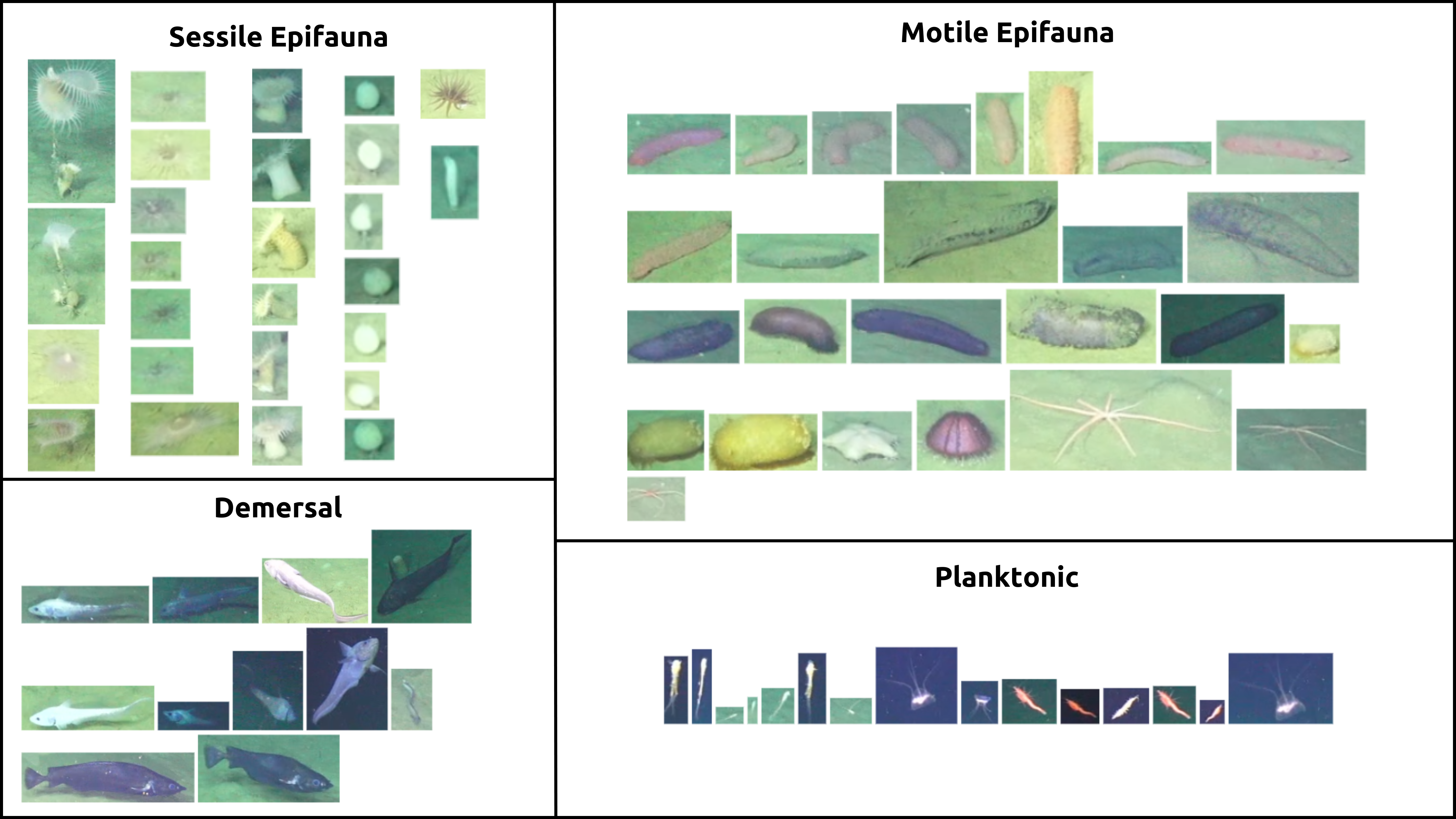
Fig. 17.1 OOI/UW/NSF Carter 2025#
To proceed:
Go into an annotation manager like Roboflow and upload the FathomNet labelmap along with your dataset. (The labelmap can be accessed on the 315 huggingface or can be automatically zipped with your dataset if you run the cell below.)
Luckily, the FathomNet model did most of the heavy lifting and should have predicted relatively close to the actual species. For each class, go through and review images with that class. As you go, mark down which of the four tiers each class best fits into. After reviewing all classes, bulk reassign the classes into the four tiers. Then, go through and check if anything was missed.
Once complete, export your dataset as a ZIP file in YOLOv11 format for further processing in the colab environment. Ensure that your splits are balanced per class before exporting! A test set will not be necessary.
import zipfile
import os
import urllib.request

def zip_folders_and_file(folder_paths, additional_file_url, output_filename):

    additional_file_path = "config.yaml"
    urllib.request.urlretrieve(additional_file_url, additional_file_path)

    with zipfile.ZipFile(output_filename, 'w', zipfile.ZIP_DEFLATED) as zipf:
        for folder in folder_paths:
            for root, _, files in os.walk(folder):
                for file in files:
                    file_path = os.path.join(root, file)
                    arcname = os.path.relpath(file_path, start=folder)
                    zipf.write(file_path, arcname)
        zipf.write(additional_file_path, os.path.basename(additional_file_path))

folders_to_zip = ["/content/frames", "/content/runs/detect/predict/labels"]
additional_file_url = "https://huggingface.co/FathomNet/MBARI-315k-yolov8/resolve/main/config.yaml?download=true"
output_zip = "/content/315k.zip"
zip_folders_and_file(folders_to_zip, additional_file_url, output_zip)
from google.colab import files

files.download('/content/315k.zip')  # Download 315k.zip
17.4. Localizing the Model#
Now that you have a finalized four-class dataset, it’s time to train a model. Use MBARI 315k as a checkpoint to import useful weights and override the old class labels with your new class labels to create a robust model tailored to your dataset.
For this training, we will select the following parameters:
Data Configuration: data.yaml, which includes the paths to your train and validation datasets.
Epochs: Set to 100 to ensure sufficient learning while avoiding overfitting.
Image Size: 1024 to balance detail and computational efficiency.
Patience: 10, to allow the model to terminate training early if no improvement is seen.
Plots: Enabled (plots=True) to generate visualizations of the training progress.
Below is the code to initiate training:
from ultralytics import YOLO

# Load a pretrained model
model = YOLO("mbari_315k_yolov8.pt")

# Train the model
results = model.train(data="data.yaml", epochs=100, imgsz=1024, plots=True, patience=10)
17.5. Tracking and Inference Parameter Adjustment#
To optimize the model, you will need to experiment with parameter combinations and evaluate performance by creating and analyzing four separate tracking videos.
17.5.1. Configure and Run Tracking#
Use the ultralytics library to configure tracking parameters. You can create four separate videos by changing the following parameters:
IoU Threshold
Confidence Threshold
Agnostic NMS
Tracker Type
Here is an example setup to guide you: Feel free to change add or delete any of the configs.
from ultralytics import YOLO

# Initialize the model
model = YOLO("/PATH/TO/YOUR/best.pt")

# Define a list of tracking configurations
tracking_configs = [
    {"conf": 0.5, "iou": 0.5, "agnostic_nms": False, "tracker": "bytetrack.yaml"},  # Default settings
    {"conf": 0.8, "iou": 0.5, "agnostic_nms": True, "tracker": "bytetrack.yaml"},   # High confidence, agnostic NMS
    {"conf": 0.3, "iou": 0.5, "agnostic_nms": False, "tracker": "sort.yaml"},       # Low confidence, SORT tracker
    {"conf": 0.5, "iou": 0.8, "agnostic_nms": True, "tracker": "sort.yaml"}         # High IoU, SORT tracker
]

# Common settings
common_settings = {
    "source": "content/transect_compressed.mp4",
    "save_txt": True,
    "imgsz": 1024
}

# Run tracking for each configuration
results = []
for config in tracking_configs:
    results.append(model.track(**common_settings, **config))
17.6. Track in Zone#
Tracking objects within a specific zone is crucial for analyzing ROV and other transects where the objects you are interested in pass by the camera. By focusing on a defined region, researchers can ensure accurate detection and counting of marine organisms or features while minimizing noise from irrelevant areas. This method helps standardize data collection, enabling more reliable comparisons across different transects and improving ecological assessments of underwater environments.
17.6.1. Video Capture Initialization#
cap = cv2.VideoCapture("/content/transect_compressed.mp4")
assert cap.isOpened(), "Error reading video file"
w, h, fps = (int(cap.get(x)) for x in (cv2.CAP_PROP_FRAME_WIDTH,
                                       cv2.CAP_PROP_FRAME_HEIGHT,
                                       cv2.CAP_PROP_FPS))
This block initializes the video capture from the specified file (transect_compressed.mp4). It verifies that the video file is successfully opened and retrieves the video’s width, height, and frames per second (fps) using OpenCV properties.
17.6.2. Video Writer Setup#
video_writer = cv2.VideoWriter("counting.avi",
                               cv2.VideoWriter_fourcc(*"mp4v"),
                               fps, (w, h))
This section sets up a video writer to save the processed frames into a new output file (counting.avi). It uses the MP4V codec for encoding and ensures the output video has the same fps and dimensions as the original.
17.6.3. Region Selection#
region_points = [(0, 576), (1024, 576), (1024, 768), (0, 768)]
This defines a rectangular region of interest (ROI) in the video, given as four coordinate points. This region is used to track and count objects only within the specified area. For our usecase the ROI is set to the bottom quarter of the video to count animals as the ROV passes above them.
17.6.4. Object Counting Initialization#
counter = solutions.ObjectCounter(
    region=region_points,
    model="/content/best.pt",
    save_txt=True,
    conf=0.10,
    iou=0.5,
    agnostic_nms=True
)
An object counter is initialized using a trained model (best.pt). The parameters include:
region=region_points: Specifies the defined tracking zone.
save_txt=True: Saves the detection results to a text file.
conf=0.10: Sets a confidence threshold of 10% for object detection.
iou=0.5: Uses a 50% Intersection Over Union (IoU) threshold to refine detections.
agnostic_nms=True: Enables class-agnostic non-maximum suppression for overlapping detections.
17.6.5. Video Processing Loop#
while cap.isOpened():
    success, im0 = cap.read()
    if not success:
        print("Video frame is empty or video processing has been successfully completed.")
        break
    im0 = counter.count(im0)  # count the objects
    video_writer.write(im0)   # write the video frames

cap.release()   # Release the capture
video_writer.release()
cv2.destroyAllWindows()
This loop processes each frame from the video:
Reads a frame from the video. If no frame is available, it prints a message and stops processing. Runs object counting on the frame using counter.count(im0). Writes the processed frame to the output video. Releases the video resources after processing all frames and closes all OpenCV windows.